Activity recognition from accelerometer data

This demo shows how the sklearn-xarray package works with the Pipeline and GridSearchCV methods from scikit-learn providing a metadata-aware grid-searchable pipeline mechansism.

The package combines the metadata-handling capabilities of xarray with the machine-learning framework of sklearn. It enables the user to apply preprocessing steps group by group, use transformers that change the number of samples, use metadata directly as labels for classification tasks and more.

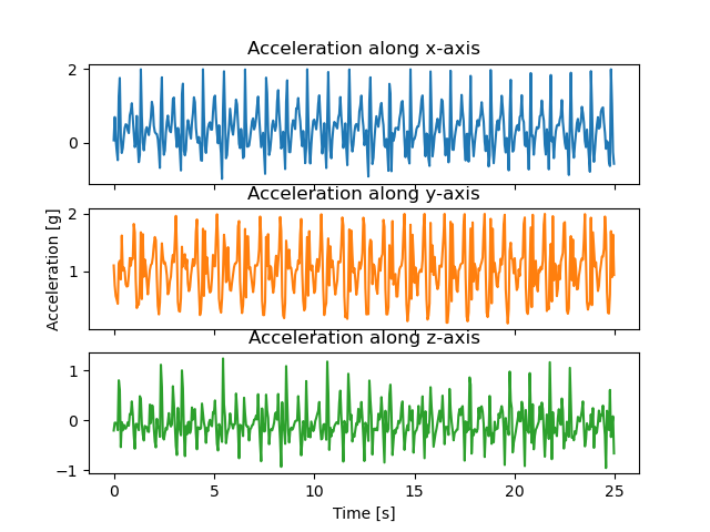
The example performs activity recognition from raw accelerometer data with a Gaussian naive Bayes classifier. It uses the WISDM activity prediction dataset which contains the activities walking, jogging, walking upstairs, walking downstairs, sitting and standing from 36 different subjects.

from __future__ import print_function

import numpy as np

from sklearn_xarray import wrap, Target
from sklearn_xarray.preprocessing import Splitter, Sanitizer, Featurizer
from sklearn_xarray.model_selection import CrossValidatorWrapper
from sklearn_xarray.datasets import load_wisdm_dataarray

from sklearn.preprocessing import StandardScaler, LabelEncoder
from sklearn.decomposition import PCA
from sklearn.naive_bayes import GaussianNB
from sklearn.model_selection import GroupShuffleSplit, GridSearchCV
from sklearn.pipeline import Pipeline

import matplotlib.pyplot as plt

First, we load the dataset and plot an example of one subject performing the ‘Walking’ activity.

Tip

In the jupyter notebook version, change the first cell to %matplotlib notebook in order to get an interactive plot that you can zoom and pan.

X = load_wisdm_dataarray()

X_plot = X[np.logical_and(X.activity == "Walking", X.subject == 1)]
X_plot = X_plot[:500] / 9.81
X_plot["sample"] = (X_plot.sample - X_plot.sample[0]) / np.timedelta64(1, "s")

f, axarr = plt.subplots(3, 1, sharex=True)

axarr[0].plot(X_plot.sample, X_plot.sel(axis="x"), color="#1f77b4")
axarr[0].set_title("Acceleration along x-axis")

axarr[1].plot(X_plot.sample, X_plot.sel(axis="y"), color="#ff7f0e")
axarr[1].set_ylabel("Acceleration [g]")
axarr[1].set_title("Acceleration along y-axis")

axarr[2].plot(X_plot.sample, X_plot.sel(axis="z"), color="#2ca02c")
axarr[2].set_xlabel("Time [s]")
axarr[2].set_title("Acceleration along z-axis")

Out:

Text(0.5, 1.0, 'Acceleration along z-axis')

Then we define a pipeline with various preprocessing steps and a classifier.

The preprocessing consists of splitting the data into segments, removing segments with nan values and standardizing. Since the accelerometer data is three-dimensional but the standardizer and classifier expect a one-dimensional feature vector, we have to vectorize the samples.

Finally, we use PCA and a naive Bayes classifier for classification.

pl = Pipeline(
    [
        (
            "splitter",
            Splitter(
                groupby=["subject", "activity"],
                new_dim="timepoint",
                new_len=30,
            ),
        ),
        ("sanitizer", Sanitizer()),
        ("featurizer", Featurizer()),
        ("scaler", wrap(StandardScaler)),
        ("pca", wrap(PCA, reshapes="feature")),
        ("cls", wrap(GaussianNB, reshapes="feature")),
    ]
)

Since we want to use cross-validated grid search to find the best model parameters, we define a cross-validator. In order to make sure the model performs subject-independent recognition, we use a GroupShuffleSplit cross-validator that ensures that the same subject will not appear in both training and validation set.

cv = CrossValidatorWrapper(
    GroupShuffleSplit(n_splits=2, test_size=0.5), groupby=["subject"]
)

The grid search will try different numbers of PCA components to find the best parameters for this task.

Tip

To use multi-processing, set n_jobs=-1.

gs = GridSearchCV(
    pl, cv=cv, n_jobs=1, verbose=1, param_grid={"pca__n_components": [10, 20]}
)

The label to classify is the activity which we convert to an integer representation for the classification.

y = Target(
    coord="activity", transform_func=LabelEncoder().fit_transform, dim="sample"
)(X)

Finally, we run the grid search and print out the best parameter combination.

if __name__ == "__main__":  # in order for n_jobs=-1 to work on Windows
    gs.fit(X, y)
    print("Best parameters: {0}".format(gs.best_params_))
    print("Accuracy: {0}".format(gs.best_score_))

Out:

Fitting 2 folds for each of 2 candidates, totalling 4 fits
[Parallel(n_jobs=1)]: Using backend SequentialBackend with 1 concurrent workers.
[Parallel(n_jobs=1)]: Done   4 out of   4 | elapsed:   12.2s finished
Best parameters: {'pca__n_components': 10}
Accuracy: 0.6746431870478216

Note

The performance of this classifier is obviously pretty bad, it was chosen for execution speed, not accuracy.